Blog

  • Hidden Markov Models: The Backwards Algorithm

    I just finished working on LEARNINGlover.com: Hidden Marokv Models: The Backwards Algorithm. Here is an introduction to the script.

    Suppose you are at a table at a casino and notice that things don’t look quite right. Either the casino is extremely lucky, or things should have averaged out more than they have. You view this as a pattern recognition problem and would like to understand the number of ‘loaded’ dice that the casino is using and how these dice are loaded. To accomplish this you set up a number of Hidden Markov Models, where the number of loaded die are the latent variables, and would like to determine which of these, if any is more likely to be using.

    First lets go over a few things.

    We will call each roll of the dice an observation. The observations will be stored in variables o1, o2, …, oT, where T is the number of total observations.

    To generate a hidden Markov Model (HMM) we need to determine 5 parameters:

    • The N states of the model, defined by S = {S1, …, SN}
    • The M possible output symbols, defined by = {1, 2, …,M}
    • The State transition probability distribution A = {aij}, where aij is the probability that the state at time t+1 is Sj, given that the state at time t is Si.
    • The Observation symbol probability distribution B = {bj(k)} where bj(k) is the probability that the symbol k is emitted in state Sj.
    • The initial state distribution = {i}, where i is the probability that the model is in state Si at time t = 0.

    The HMMs we’ve generated are based on two questions. For each question, you have provided 3 different answers which leads to 9 possible HMMs. Each of these models has its corresponding state transition and emission distributions.

    • How often does the casino change dice?
      • 0) Dealer Repeatedly Uses Same Dice
      • 1) Dealer Uniformly Changes Die
      • 2) Dealer Rarely Uses Same Dice
    • Which sides on the loaded dice are more likely?
      • 0) Larger Numbers Are More Likely
      • 1) All Numbers Are Randomly Likely
      • 2) Smaller Numbers Are More Likely
    How often does the casino change dice?
    Which sides on
    the loaded dice
    are more likely?
    (0, 0) (0, 1) (0, 2)
    (1, 0) (1, 1) (1, 2)
    (2, 0) (2, 1) (2, 2)

    One of the interesting problems associated with Hidden Markov Models is called the Evaluation Problem, which asks the question “What is the probability that the given sequence of observations O = o1, o2, …, oT are generated by the HMM . In general, this calculation, p{O | }, can be calculated by simple probability. However because of the complexity of that calculation, there are more efficient methods.

    The backwards algorithm is one such method (as is the forward algorithm). It creates an auxiliary variable t(i) which is the probability that the model has generated the partially observed sequence ot+1, …, oT, where 1 t T. This variable can be calculated by the following formula:

    t(i) = j = 1 to N(t+1(j) * aij * bj(ot+1))

    We also need that T(i) = 1, for 1 i N.

    Once we have calculated the t(j) variables, we can solve the evaluation problem by p{O | } i = 1 to N1(i)

    There is more on this example at LEARNINGlover.com: Hidden Marokv Models: The Backwards Algorithm.

    Some further reading on Hidden Markov Models:

  • Hidden Markov Models: The Forward Algorithm

    I just finished working on LEARNINGlover.com: Hidden Marokv Models: The Forward Algorithm. Here is an introduction to the script.

    Suppose you are at a table at a casino and notice that things don’t look quite right. Either the casino is extremely lucky, or things should have averaged out more than they have. You view this as a pattern recognition problem and would like to understand the number of ‘loaded’ dice that the casino is using and how these dice are loaded. To accomplish this you set up a number of Hidden Markov Models, where the number of loaded die are the latent variables, and would like to determine which of these, if any is more likely to be using.

    First lets go over a few things.

    We will call each roll of the dice an observation. The observations will be stored in variables o1, o2, …, oT, where T is the number of total observations.

    To generate a hidden Markov Model (HMM) we need to determine 5 parameters:

    • The N states of the model, defined by S = {S1, …, SN}
    • The M possible output symbols, defined by = {1, 2, …, M}
    • The State transition probability distribution A = {aij}, where aij is the probability that the state at time t+1 is Sj, given that the state at time t is Si.
    • The Observation symbol probability distribution B = {bj(k)} where bj(k) is the probability that the symbol k is emitted in state Sj.
    • The initial state distribution = {i}, where i is the probability that the model is in state Si at time t = 0.

      The HMMs we’ve generated are based on two questions. For each question, you have provided 3 different answers which leads to 9 possible HMMs. Each of these models has its corresponding state transition and emission distributions.

      • How often does the casino change dice?
        • 0) Dealer Repeatedly Uses Same Dice
        • 1) Dealer Uniformly Changes Die
        • 2) Dealer Rarely Uses Same Dice
      • Which sides on the loaded dice are more likely?
        • 0) Larger Numbers Are More Likely
        • 1) All Numbers Are Equally Likely
        • 2) Smaller Numbers Are More Likely
      How often does the casino change dice?
      Which sides on
      the loaded dice
      are more likely?
      (0, 0) (0, 1) (0, 2)
      (1, 0) (1, 1) (1, 2)
      (2, 0) (2, 1) (2, 2)

      One of the interesting problems associated with Hidden Markov Models is called the Evaluation Problem, which asks the question “What is the probability that the given sequence of observations O = o1, o2, …, oT are generated by the HMM . In general, this calculation, p{O | }, can be calculated by simple probability. However because of the complexity of that calculation, there are more efficient methods.

      The forward algorithm is one such method. It creates an auxiliary variable t(i) which is the probability that the model has generated the partially observed sequence o1, …, ot, where 1 t T. This variable can be calculated by the following formula:

      t+1(j) = bj(ot+1)i = 1 to N(t(i)aij), where 1 j N, 1 t T-1.

      1(j) = jbj(o1), for 1 j N.

      Once we have calculated the t(j) variables, we can solve the evaluation problem by p{O | } = i = 1 to N T(i)

      There is more on this example at LEARNINGlover.com: Hidden Marokv Models: The Forward Algorithm.

      Some further reading on Hidden Markov Models:

  • Term Frequency Inverse Document Frequency

    TFIDF Example Page

    I recently found myself at a gathering where there was a presentation followed by a question and answer session. The presenter spoke about how recent advents in technology had allowed for questions to be submitted online, which led to many more questions than they normally receive. He then stated that rather than attempt to answer each question individually, that the questions would be grouped together to attempt to cover as many areas as possible. I must say that while the presentation and the Q & A sessions in themselves were informative, I was probably most excited when I heard the speaker present this problem. I immediately began analyzing the problem, developing a strategy and decided to speak with the presenter afterwards.

    I like to think of three trains of thought when it comes to computers. There are those who watch science fiction movies and believe that computers can do literally anything; there are those who haven’t seen computers tackle complex tasks, so they think of computers as simple “adding machines”; and then there are those of us who work with computers on a day to day basis. There is an extremely long list of things that computers can do – a list which far outnumbers the things that people in the second category try to limit computers to. However, the fact that computers have not gotten to an “I, Robot” mentality does not make them useless.

    As a case in point, one of the more popular and thus more important areas of data mining is that of text analytics. This area attempts to combine the fields of computer science and natural language processing to build tools that gather meaning from text documents. Several algorithms have emerged in this field and the one I choose to write about today is the Term Frequency Inverse Document Frequency Matrix. This is the means by which I suggested to help with the question and answer session I mentioned earlier.

    The Term Frequency Inverse Document Frequency (TF-IDF) Matrix considers as input a list of documents. Each of these documents consists of words (or terms). Two important things are computed for each term, the “term frequency” and the “inverse document frequency”. There are several ways to compute each of these, but the most basic way of computing each is to let the term frequency of a given word and document tf(w, d) be the number of times the word w appears in the document d. In a similar manner, the inverse document frequency idf(w, D) tells how common the word w is across all the documents d \in D. The calculation of the TF-IDF matrix consists of creating a column corresponding to each word and a row for each document. The tf and idf values are then computed for each cell and the value in the cell is the product tf(w, d)*idf(w, D).

    Once the TF-IDF matrix has been computed, we can use a metric like Cosine Similarity to determine how similar two documents are. When every pair of document is compared using the cosine similarity metric, it forms a similarity matrix that shows how the documents relate to one another. This matrix can be clustered via k-means clustering or hierarchal clustering show the similar documents.

    I’ve written a script which considers a set of quotations and randomly displays a set of those quotations and uses the TF-IDF matrix to determine how similar these quotations are. Let me know what you think.

  • Covariance of Vectors

    Covariance Image Link

    Most of the things we think about have many different ways we could describe them. Take for example a movie. I could describe a movie by its genre, its length, the number of people in the movie, the number of award winners, the length of the explosions, the number of fight scenes, the number of scenes, the rating it was given by a certain critic, etc. The list goes on and on. How much do these things influence one another? How likely is a person to enjoy a movie? Is that related to the number of award winners in the movie? Answering this type of a question can often help understand things like what might influence a critics rating or more importantly which movies are worth my $15 ticket price.

    Movies are just one example of this. Other areas like sports, traffic congestion, or food and a number of others can be analyzed in a similar manner. With data becoming available at unprecedented rates and areas like cloud computing and data science becoming key buzzwords in industry, the ability to understand these relationships is becoming more and more important.

    As a mathematician, I enjoy being able to say with certainty that some known truth is the cause of some other known truth, but it not always easy (or even possible) to prove the existence of such a relationship. We are left instead with looking at trends in data to see how similar things are to one another over a data set. Measuring the covariance of two or more vectors is one such way of seeking this similarity.

    Before delving into covariance though, I want to give a refresher on some other data measurements that are important to understanding covariance.
    – Sum of a vector:
    If we are given a vector of finite length we can determine its sum by adding together all the elements in this vector. For example, consider the vector v = (1, 4, -3, 22). Then sum(v) = 1 + 4 + -3 + 22 = 24.

    – Length of a vector:
    If we are given a vector of finite length, we call the number of elements in the vector the length of the vector. So for the example above with the vector v = (1, 4, -3, 22), there are four elements in this vector, so length(v) = 4.

    – Mean of a vector:
    The mean of a finite vector is determined by calculating the sum and dividing this sum by the length of the vector. So, working with the vector above, we already calculated the sum as 24 and the length as 4, which we can use to calculate the mean as the sum divided by the length, or 24 / 4 = 6.

    – Variance of a vector:
    Once we know the mean of a vector, we are also interested in determining how the values of this vector are distributed across its domain. The variance measures this by calculating the average deviation from the mean. Here we calculate the deviation from the mean for the ith element of the vector v as (vi)2. We can get the average deviation from the mean then by computing the average of these values.

    So if the vector v has n elements, then the variance of v can be calculated as Var(v) = (1/n)i = 1 to n((vi)2).

    Once again dealing with the vector above with v = (1, 4, -3, 22), where the mean is 6, we can calculate the variance as follows:

    vi vi (vi)2
    1 -5 25
    4 -2 4
    -3 -9 81
    22 16 256

    To calculate the mean of this new vector (25, 4, 81, 324), we first calculate the sum as 25 + 4 + 81 + 256 = 366. Since the length of the new vector is the same as the length of the original vector, 4, we can calculate the mean as 366 / 4 = 91.5

    The covariance of two vectors is very similar to this last concept. Instead of being interested in how one vector is distributed across its domain as is the case with variance, covariance is interested in how two vectors X and Y of the same size are distributed across their respective means. What we are able to determine with covariance is things like how likely a change in one vector is to imply change in the other vector. Having a positive covariance means that as the value of X increases, so does the value of Y. Negative covariance says that as the value of X increases, the value of Y decreases. Having zero covariance means that a change in the vector X is not likely to affect the vector Y.

    With that being said, here is the procedure for calculating the covariance of two vectors. Notice that it is very similar to the procedure for calculating the variance of two vectors described above. As I describe the procedure, I will also demonstrate each step with a second vector, x = (11, 9, 24, 4)

    1. Calculate the means of the vectors.
    As we’ve seen above, the mean of v is 6.
    We can similarly calculate the mean of x as 11 + 9 + 24 + 4 = 48 / 4 = 12

    2. Subtract the means of the vectors from each element of the vector (xiX) and (YiY).

    We did this for v above when we calculated the variance. Below are the values for v and for x as well.

    vi – meanv

    -5

    -2

    -9

    16

    i vi xi xi – meanx
    1 1 11 -1
    2 4 9 -3
    3 -3 24 12
    4 22 4 -8

    3. For each element i, multiply the terms (xiX) and (YiY).

    This gives us the following vector in our example:
    (-5)(-1), (-2)(-3), (-9)(12), (16)(-8) = (5, 6, -108, -128).

    4. Sum the elements obtained in step 3 and divide this number by the total number of elements in the vector X (which is equal to the number of elements in the vector Y).

    When we sum the vector from step 3, we wind up with 5 + 6 + -108 + -128 = -225
    And the result of dividing -225 by 4 gives us -225/4 = – 56.25.

    This final number, which for our example is -56.25, is the covariance.

    Some important things to note are

    • If the covariance of two vectors is positive, then as one variable increases, so does the other.
    • If the covariance of two vectors is negative, then as one variable increases, the other decreases.
    • If the covariance of two vectors is 0, then one variable increasing (decreasing) does not impact the other.
    • The larger the absolute value of the covariance, the more often the two vectors take large steps at the same time.
    • A low covariance does not necessarly mean that the two variables are independent. I’ll give a quick example to illustrate that.
      Consider the vectors x and y given by x = (-3, -2, -1, 0, 1, 2, 3) and y = (9, 4, 1, 0, 1, 4, 9).
      The mean of x is 0, while the mean of y is 7.
      The mean adjusted values are (-3, -2, -1, 0, 1, 2, 3) and (2, -3, -6, -7, -6, -3, 2).
      The product of these mean adjusted values is (-6, 6, 6, 0, -6, -6, 6).
      If we sum this last vector, we get 0, which after dividing by 7 still gives a value of 0.
      So the covariance of these two vectors is 0.

      We can easily see that for each value xi in x, the corresponding yi is equal to xi2

    I have written a script to help understand the calculation of two vectors.

  • The Gram-Schmidt Process and Orthogonal Vectors

    Suppose I gave you some red fingerpaint and asked you to make all the colors you could from this paint. You’d probably come up with a diverse collection of pinks, reds and burgendys – going through the range of reds – but you would be unable to produce a color that does not depend solely on red, like purple.

    Shades of Red

    If I were to ask you to produce purple, your reply may be something like “well, give me blue and I’ll be able to color in purple”. When we think in terms of colors, it is easy to understand the concept of the span of a set of colors. In this context, span refers to the set of colors we can create from our original colors.

    Now, lets think in terms of numbers (actually vectors) instead of colors. If I gave you a similar task as above, but instead of the color red, I gave you the vector (1, 0, 0) and told you to see what other numbers you could get from this (by scalar multiplication and the addition of any two vectors already produced) then you would probably come back to me and show me how you could use the vector (1, 0, 0) to produce the entire real number line in that first dimension, but leaving the other coordinates at 0.

    If (similar to the color example) I asked you to use the vector (1, 0, 0) to produce the vector (1, 1, 0), then you may reply with a similar statement as above: “you give me the vector (0, 1, 0) and I’ll produce (1, 1, 0)”. That’s because the vectors (1, 0, 0) and (1, 1, 0) are linearly independent. This is a mathematical way of saying what we’ve already stated, that you cannot get one vector as a scalar multiple of the other vector for any real number scalar.

    If two vectors are linearly independent then neither one belongs to the span of the other. Just as you cannot create blue from red, you cannot create red from blue. So this means that if I were to give you the colors red and blue, then the set of colors that you can create has increased from what you could create from either only red or only blue. Similarly, the vector sets {(1, 0, 0), (0, 1, 0)} spans more vectors than just {(1, 0, 0)} or {(0, 1, 0)}.

    Consider then the following two sets of vectors: {(1, 0, 0), (0, 1, 0)} and {(1, 0, 0), (1, 1, 0)}. Notice that (1, 1, 0) [belongs to] span({(1, 0, 0), (0, 1, 0)}) because (1, 1, 0) = (1, 0, 0) + (0, 1, 0). Likewise (0, 1, 0) [belongs to] span({(1, 0, 0), (1, 1, 0) because (0, 1, 0) = (1, 1, 0) – (1, 0, 0). So we can see that these two sets span the same sets of vectors. But which is a better set to use?

    Lets to back to colors and think of the set {red, purple}. Here we can think of purple as a simple combination of red and blue (i.e. purple = red + blue). What happens if we mix red and purple? If we think of it in terms of an axis, the fact that purple contains red in it means that as we walk along the purple axis, we are walking along the red axis as well. If we considered the set {red, blue}, we see that this is not happening. As we change the amount of red in our color, the amount of blue is unaffected. Likewise, if we change the amount of blue, the amount of red is not affected. If we were to draw these axes, we could see that this happens because the colors red and blue are perpendicular (or orthogonal) to one another, while red and purple are not.

    Color Axis Example

    Replacing these colors with vectors again, we get the same thing. We have the option of using the vector set {(1, 0, 0), (1, 1, 0)} or {(1, 0, 0), (0, 1, 0)} as our axis and it is better to use the second set because the two vectors are not just independent of one another, but also are at a 90[degree] angle, or are orthogonal to one another.

    When given a set of vectors (or a set of colors), an important problem is to determine the span of those vectors and to be able to produce an orthogonal set of vectors that spans that same space. The Gram-Schmidt process provides a procedure for producing these orthogonal vectors.

    The way the procedure works is to build an orthogonal set of vectors from the original set by computing the projection of the current vector being worked on in terms of the previous vectors in the orthogonal set. This projection procedure is defined as proju(v) = (u, v / u, u)u. The formula for the ith vector of the Gram-Schmidt process is

    ui = vij = 1 to i-1 projuj(vi).

    Here is a script I’ve written to help with this process.

  • Permutation Problems

    I love to play with puzzles. When I was in grade school I would spend hours at a time figuring out ways to solve from things like Tetris, Mindsweeper, Solitare, and Freecell. Later I was introduced to puzzles involving numbers like Sudoku and Nonograms.

    These puzzles are often interesting in part because there is generally a very large way that things can be arranged, but only a few of these arrangements are correct. Generally a person solving a puzzle will figure out certain things that must be true or cannot be true, which helps in solving the puzzle and reducing the number of possible cases. Initially, though, we are often left with a situation where we have a new puzzle and our only method is to keep trying every possible solution until we start to notice a pattern (or reach a solution).

    For example, consider a Sudoku puzzle. We are given a partially filled in grid and our job is to fill in the remaining cells with the rules that every row, column and marked subgrid must have the numbers 1 – 9 exactly once. One initial attempt at solving such a puzzle could be to attempt to permute the string 1, 2, 3, 4, 5, 6, 7, 8, 9 until we find a solution that fits the first row, then do the same with the second row, and so on and so forth.

    One immediate question is how many ways are there to permute the numbers 1, …, 9? We can answer this by realizing that each permutation is a new string. So for each string that we construct, we have 9 choices for the first element in the string. Then once that element has been chosen, we are not allowed for that element to appear anywhere else. So there are only 8 possible choices for what can go in the second string. Continuing this process, we see that the number of possible permutations we can construct from the string 1, …, 9 is

    9 * 8 * 7 * 6 * 5 * 4 * 3 * 2 * 1 = 362880

    This is a large number of possible strings to generate just to get one row of a Sudoku, so hopefully you’ll be able to notice the pattern before going through this whole set (because once you’ve generated the first row you still have to do the other 8 rows).

    Nonetheless because there is often great value that can be gained by knowing how to permute through all possible solutions, I have written three functions that help with this process: Next_Permutation, Previous_Permutation, and Random_Permutation.

    Before I give these algorithms, I want to highlight two notations on ordering string. A string (a1, a2, …, an) is said to be in lexicographical order (or alphabetical order) if for each i [in] 1, …, n-1, ai [<=] ai+1. Likewise, a string is said to be in reverse lexicographical order if for each i [in] 1, …, n-1, ai [>=] ai+1.

    Next Permutation

    If the given string is not in reverse lexicographic order, then there exists two elements j1 and j2 such that j1 [<] j2 and aj1 [<] aj2.
    1. The Next_Permutation algorithm first searches for the largest element j1 such that aj1 [<] aj1 + 1. Since we said the string is not in reverse lexicographic order, this j1 must exist.
    2. Once this j1 is found, we search for the smallest element aj2 such that aj2 [>] aj1. Again, since we know that this is true for j1 + 1, we know that such a j2 must exist.
    3. We swap the elements aj1 and aj2.
    4. The elements after j1 + 1 are then placed in lexicographic order (i.e. in order such that ai [>=] ai+1

    If the given string is in reverse lexicographic order, then we simply reverse the string.

    Previous Permutation

    If the given string is not in lexicographic order, then there exists two elements j1 and j2 such that j1 [<] j2 and aj1 [>] aj2.
    1. The Previous_Permutation algorithm first searches for the largest element j1 such that aj1 [>] aj1 + 1. Since we said the string is not in reverse lexicographic order, this j1 must exist.
    2. Once this j1 is found, we search for the smallest element aj2 such that aj1 [>] aj2. Again, since we know that this is true for j1 + 1, we know that such a j2 must exist.
    3. We swap the elements aj1 and aj2.
    4. The elements after j1 + 1 are then placed in reverse lexicographic order (i.e. in order such that ai [<=] ai+1

    If the given string is in lexicographic order, then we simply reverse the string.

    Random Permutation

    This generates a random string permutation.

    This script can be seen here, set to work on permutations of colors.

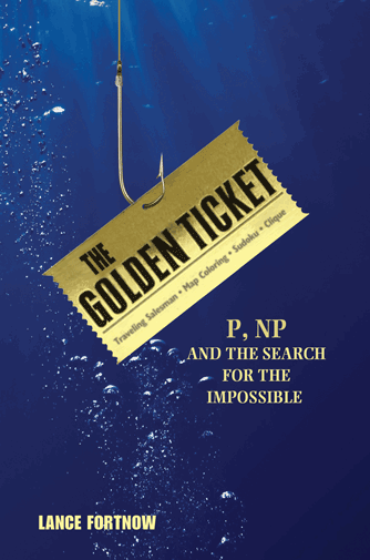
  • My Review of “The Golden Ticket: P, NP, and the Search for the Impossible”

    The Golden Ticket Image

    I came home from work on Wednesday a bit too tired to go for a run and a bit too energetic to sit and watch TV. So I decided to pace around my place while reading a good book. The question was did I have a good book to read. I had been reading sci-fi type books earlier this month and wanted a break from that, so I looked in my mailbox and noticed that I had just received my copy of “The Golden Ticket: P, NP, and the Search for the Impossible“. At the time, I was of the mindset that I had just gotten off of work and really didn’t want to be reading a text book as if I was still at work. But I decided to give it a try and at least make it through the first few pages and if it got to be overwhelming, I’d just put it down and do something else.

    About three hours later I was finishing the final pages of the book and impressed that the author (Lance Fortnow) was able to treat complexity theory the same way that I see physics professors speaking about quantum physics and the expanding universe on shows like “the Universe” and “Through the Wormhole with Morgan Freeman” where complex topics are spoken about with everyday terminology. It wouldn’t surprise me to see Dr. Fortnow on shows like “The Colbert Report” or “The Daily Show” introducing the topics in this book to a wider audience.

    Below is the review I left on Amazon.

    I really enjoyed this book. It was a light enough read to finish in one sitting on a weeknight within a few hours, but also showed its importance by being able to connect the dots between the P = NP problem to issues in health care, economics, security, scheduling and a number of other problems. And instead of talking in a "professor-like" tone, the author creates illustrative examples in Chapters 2 and 3 that are easy to grasp. These examples form the basis for much of the problems addressed in the book.

    This is a book that needed to be written and needs to be on everyone's bookshelf, particularly for those asking questions like "what is mathematics" or "what is mathematics used for". This book answers those questions, and towards the end gives examples (in plain English) of the different branches of mathematics and theoretical computer science, without making it read like a text book.

    Also, here is a link to the blog that Lance Fortnow and William Gasarch run called “Computational Complexity”, and here is a link to the website of the book, “The Golden Ticket: P, NP, and the Search for the Impossible”

  • Approximating the Set Cover Problem

    Set Cover Problem Instance

    I just finished my weekly task of shopping for groceries. This can be a somewhat daunting task because I generally have a list of things that I’ll need which cannot all be purchased at a single location. What often happens is that I find that many of the items on my list are ONLY offered at certain stores – generic brands of certain items for example. My goal then changes from minimizing the total amount of money spent to minimizing the number of stores that I must visit to purchase all of my items.

    To formulate this as a mathematical problem, suppose that I have a grocery list of items I would like to buy, represented by the lists item1, item2, …, itemn, where n represents the number of items I have on this list. Suppose also that there are stores Store1, Store2, …, Storem (each one distinct) that offer some combination of items I have on my list. What I would like to do is minimize the number of stores I have to visit to purchase these items.

    The problem I just described is famous because it is one that many people face on a regular basis. In a more general form, it is so famous that it has a name for it, called the Set Cover Problem (or the Minimum Set Cover Problem). In the general form of this problem, we replace the grocery list with a set of items called our universe. The lists of items offered at each store are the collections of subsets of the universe. In the problem, as in the example above, we would like to select enough subsets from this collection that we are able to obtain every element in our universe. We would like to do this with as low a number of sets as possible.

    In my previous post, I described the 21 problems that Karp proved were NP-Complete. Set Cover was one of those problems, showing that this is a hard problem to solve. What I will do is introduce three ways to reach a near-optimal solution relatively quickly.

    Greedy Method

    One of the first approaches one may take to solve this problem is to repeatedly select the subset that contains the most new items. That’s how the greedy approach to set cover operates. The method knows to terminate when all elements belong to one of the selected sets. In the shopping example above, this would be accomplished by visiting the store that had the most items on my list and purchasing those items at this store. Once this is done, the items that have been purchased can be crossed off my list and we can visit the store with the most items on my remaining list, stopping when the list is empty.

    Linear Programming Relaxation

    Instead of stating the set cover problem with words, there is a way of describing the situation with mathematical inequalities. For instance, suppose that the soap I like to purchase is only available at stores Store1, Store4 and Store9. Then I could introduce a variable xi for each store i and the requirement that I purchase this soap can be restated as :

    x1 + x4 + x9 greater than or equals 1

    Because we can either purchase some items or not purchase these items, each variable xi is 0 or 1 (called a binary variable). We can introduce similar constraints for each element in our universe (or on our grocery list). These inequalities (called constraints) have the form:

    for each element e in U, sumi | e in Si xi greater than or equals 1

    Our goal of minimizing the number of sets chosen (stores visited) can be stated by the objective function:
    minimize sum1 less than or equals i less than or equals n xi

    So the mathematical formulation for this problem can be stated as

    minimize sum1 less than or equals i less than or equals n xi
    Subject to
    for each element e in U, sumi | e in Si xi greater than or equals 1
    for each set i, xi in {0, 1}.

    Formulations of this type, where variables are restricted to a finite set (in this case the x variables being either 0 or 1) are called integer programs. Unfortunately, there is no easy way to solve these formulations either. However, there is a related problem which can be solved quickly.

    Instead of restricting the x variables to the values of 0 or 1, we could allow them to take on any value within this range, i.e. 0 less than or equals xi less than or equals 1 for each set Si. Doing this converts the problem from an integer programming problem into a linear programming problem (called the LP-Relaxation), which can be solved quickly. The issue with this method though is that the solution obtained by an LP-Relaxation is not guaranteed to be an integer. In this case, how do we interpret the values xi?

    Randomized Rounding Method

    One approach to dealing with a non-integer solution to the LP-Relaxation is to treat the xi values as probabilities. We can say that xi is the probability that we select set i. This works because each value of xi is in the range of 0 to 1, which is necessary for a probability. We need to repeatedly select sets with their associated probabilities until all elements in our universe are covered. Selecting our sets based on this procedure is the randomized rounding approach.

    Deterministic Rounding Method

    A second approach to dealing with a non-integer solution to the LP-Relaxation is to base our solution on the most occurring element. If we let f be this frequency (i.e.the number of sets that the most occurring element occurs in), then we can define a solution by selecting set i if the LP=Relaxation solution gives the variable xi a value of at least (1/f).

    None of these three approaches is guaranteed to give an optimal solution to an instance of this problem. I will not go into it in this post, but these can all be shown to be within some guaranteed range of the optimal solution, thus making them approximation algorithms.

    You can see how the three algorithms compare on random problem instances here.

    Hope you enjoy.

  • What is a “Hard” Problem?

    Throughout our lives, we are introduced to a wide variety of problems. Naturally we tend to think of some problems as more difficult than others. If you were doing the exercises at the end of a chapter in a book, the author generally tends to begin with those exercises that can be completed in a few minutes or directly from the material in the chapter. The exercises in the end tend to be more time consuming and possibly require outside resources. In this sense, these authors tend to compare the difficulty of problems by the amount of time they expect the average reader to take to solve them.

    This is a popular way to look at difficulty – in terms of how difficult it is for not only a single person to solve a problem (say you or I), but how long it would take our peers as well as yourself to solve the problem. But how can we measure this? Should I assume that because a problem takes me two years to solve that it would take the average person the same amount of time? Or, if a problem has never been solved, is that because of the difficulty of the problem or could it be for another reason like because no-one had thought of the problem before?

    In particular, these questions were being asked in the world of computer science in the 1960s and 1970s. It was around this time that Stephen Cook came up with the concept being able to compare how difficult one problem was in comparison to another. A problem A can be “reduced” to another problem B if a way to solve problem B quickly also gives way to a way to solve problem A quickly.

    This concept of reducibility provided a foundation for this concept of difficulty as it was no longer enough to say “I think this problem is hard”, or “the average person would take just as long as me to solve this problem”. No, instead, Cook considered problems that many thought were difficult and showed that the satisfiability problem (the question of whether a given boolean formula contains an assignment to the variables that satisfies all the clauses) could be used to show that all quickly verifiable decision problems (also called problems in NP), where the instances with a “yes” answer have short proofs of the fact that the answer is indeed “yes” could be reduced to this problem.

    This meant that the satisfiability problem was at least as hard as every one of these quickly verifiable decision problems, so if this problem could be solved quickly, then every one of these quickly verifiable decision problems could also be solved quickly. So the satisfiability problem is at least as hard as every problem in this class, NP. We call such problems that have this property NP-Hard. Decision Problems that are NP-Hard are called NP-Complete. Richard Karp later published a paper that proposed 21 NP-Complete problems, one of which was the Knapsack Problem I spoke about last time.

    Garey Johnson NP-Complete Image

    This concept of NP-Complete gives light to the image that became famous in the book by Garey and Johnson “Computers and Intractability: A Guide to the Theory of NP-Completeness”. It shows that the concept of difficulty still builds on the ability of our peers to solve a given problem. But by introducing a class of “hard” problems, and a litmus test for inclusion into that class, researchers could now consider new problems and determine their difficulty by comparing it to known hard problems.

    (a quick note. I’ve used the term “quickly” here, but the formal phrase that I mean by that is that the problem is solvable by an algorithm whose worse case running time is bounded by a polynomial on the input parameters of the problem)

    Other Blogs that have covered this topic:
    Explorations
    To Imaging, and Beyond!

  • Knapsack Problems

    Knapsack Image

    I have added a script to help users understand the knapsack problem as well as some attempts at solving it.

    To help understand this problem, I want you to think about a common situation in many people’s lives. You have a road trip coming up today and you’ve overslept and are at risk of missing your flight. And to top matters off, you were planning to pack this morning but now do not have the time. You quickly get up and begin to get ready. You grab the first bag you see and quickly try to make decisions on which items to take. In your head you’re trying to perform calculations on things you’ll need for the trip versus things that you can purchase when you get there; things that you need to be able to have a good time versus things you can do without. And to top matters off, you don’t have time to look for your ideal luggage to pack these things. So you have the additional constraint that the items you pick must all fit into this first bag you found this morning.

    The situation I described above is a common problem. Even if we ignore the part about the flight, and just concentrate on the problem of trying to put the most valuable set of items in our bag, where each item has its own value and its own size limitations, this is a problem that comes up quite often. The problem is known (in the math, computer science and operations research communities) as the knapsack problem. It is known to be difficult to solve (it is said to be NP-Hard and belongs to a set of problems that are thought to be the most difficult problems within its class). Because of this difficulty, this problem has been well studied.

    What I provide in my script are two approaches to solving this problem. The first is a greedy approach, which selects a set of items by iteratively choosing the item with the highest remaining value to size ratio. This approach solves very fast, but can be shown to give sub-optimal solutions.

    The second approach is a dynamic programming approach. This algorithm will solves the problem by ordering the items 0, 1, …, n and understanding that in order to have the optimal solution on the first i items, the optimal solution must have been first selected on the fist i-1 items. This algorithm will optimally solve the problem, but it requires the computation of many sub-problems which causes it to run slowly.

    Update (4/2/2013): I enjoy this problem so much that I decided to implement two additional approaches to the problem: Linear Programming and Backtracking.

    The Linear Programming approach to this problem comes from the understanding that the knapsack problem (as well as any other NP-Complete problem) can be formulated as an Integer Program (this is a mathematical formulation where we seek to maximize a linear objective function subject to a set of linear inequality constraints with the condition that the variables take on integer values). In the instance of the knapsack problem we would introduce a variable xi for each item i; the objective function would be to maximize the total value of items selected. This can be expressed as a linear objective function by taking the sum of the products of the values of each item vi and the variable xi; the only constraint would be the constraint saying that all items fit into the knapsack. This can be expressed as a linear inequality constraint by taking the sum of the products of the weights of each item wi and the variable xi. This sum can be at most the total size of the knapsack. In the integer programming formulation, we either select an item or we do not. This is represented in our formulation by allowing the variable xi = 1 if the item is selected, 0 otherwise.

    The LP relaxation of an integer program can be found by dropping the requirements that the variables be integer and replacing them with linear equations. So in the case of the knapsack problem, instead of allowing the variables to only take on values of 0 and 1, we would allow the variables to take on any value in the range of 0 and 1, i.e 0 <= xi <= 1 for each item i. We can then solve this LP to optimality to get a feasible solution to the knapsack problem. The second knapsack approach I implemented today is through backtracking. Similar to the Dynamic Programming approach to this problem, the backtracking approach will find an optimal solution to the problem, but these solutions generally take a long time to compute and are considered computationally inefficient. The algorithm I implemented here first orders the item by their index, then considers the following sub-problems for each item i "What is the best solution I can obtain with this initial solution?". To answer this question, the algorithm begins with an initial solution (initially, the empty set) and a set of unchecked items (initially, all items) and recursively calls itself on sub-problems with an additional item as a part of the initial solution and with this item removed from the unchecked items. So check out my knapsack problem page. I think its a good way to be introduced to the problem itself, as well as some of the techniques that are used in the fields of mathematics, computer science, engineering and operations research.

    Other Blogs covering this topic:
    Journey to the Four Point Oh